Density plot tutorial

One of the most useful tools in MultiMin is the visualization of the probability density of a data distribution. In this tutorial, you will learn how to use the DensityPlot class and its most interesting features, not only for viewing data but also for visualizing the probability density of a data distribution.

Installation and importing

If you’re running this in Google Colab or need to install the package, uncomment and run the following cell:

[1]:

try:
    from google.colab import drive
    %pip install -Uq multimin
except ImportError:
    print("Not running in Colab, skipping installation")
    %load_ext autoreload
    %autoreload 2
!mkdir -p gallery/

# Uncomment to install from GitHub (development version)
# !pip install git+https://github.com/seap-udea/MultiMin.git

Not running in Colab, skipping installation

[2]:

import multimin as mn
mn.show_watermark = True

import matplotlib.pyplot as plt
import plotly.graph_objects as go

import numpy as np
import pandas as pd
np.random.seed(1)
deg = np.pi/180

import warnings
warnings.filterwarnings("ignore")

figprefix = "multiplot"

Welcome to MultiMin v0.11.2. ¡Al infinito y más allá!

Real data

multimin was originally developed to solve the problem of describing the distribution of asteroids in the space of orbital elements. This is a true scientific application of the package that illustrate the power of the methods and the versatility of the numerical methods provided by the package.

Load the dataset (e.g. orbital elements):

[3]:

# NEA Data
df_neas=pd.read_json(mn.Util.get_data("nea_data.json.gz"))

# Let's filter 10000 asteroids
df_neas=df_neas.sample(10000)

# Let's select the columns we want to fit
df_neas["q"]=df_neas["a"]*(1-df_neas["e"])
data_neas=np.array(df_neas[["q","e","i","Node","Peri","M"]])

Representing the data

To create a graphical representation of a dataset like data_neas, the first thing we need is a description of the variables:

[4]:

properties=dict(
    q=dict(label=r"$q$ [au]",range=[0.0,1.3]),
    e=dict(label=r"$e$",range=[0.0,1.0]),
    i=dict(label=r"$I$ [deg]",range=[0.0,180.0]),
    W=dict(label=r"$\Omega$ [deg]",range=[0,360]),
    w=dict(label=r"$\omega$ [deg]",range=[0,360]),
)

Now we must instantiate the MultiPlot object:

[5]:

G=mn.MultiPlot(properties,figsize=2)

../_images/examples_multimin_density_plot_tutorial_13_0.png

Once the MultiPlot object is instantiated, we can add content to it. There are 4 methods to do so:

sample_scatter: Adds a scatter plot of a random sample.
sample_hist: Adds a histogram of a random sample.
mog_pdf: Adds the density of the Gaussian mixture.
mog_contour: Adds the contour of the Gaussian mixture.

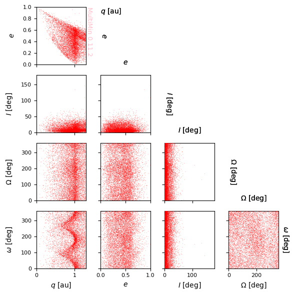
Por ejemplo para mostrar la distribución de elementos orbitales:

[6]:

G=mn.MultiPlot(properties,figsize=1.5)

sargs=dict(s=0.2,edgecolor='None',color='r')
scatter=G.sample_scatter(data_neas,**sargs)

plt.savefig(f'gallery/{figprefix}_data_neas.png')

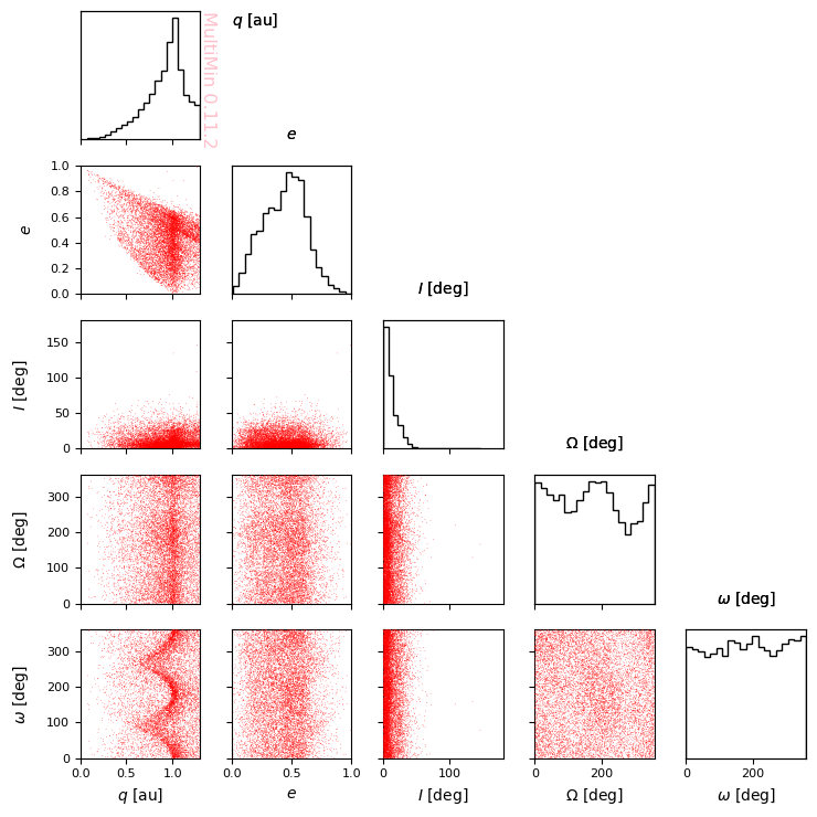
../_images/examples_multimin_density_plot_tutorial_16_0.png

You can add marginal plots:

[7]:

G=mn.MultiPlot(properties,figsize=1.5,marginals=True)

sargs=dict(s=0.2,edgecolor='None',color='r')
scatter=G.sample_scatter(data_neas,**sargs)

plt.savefig(f'gallery/{figprefix}_data_neas.png')

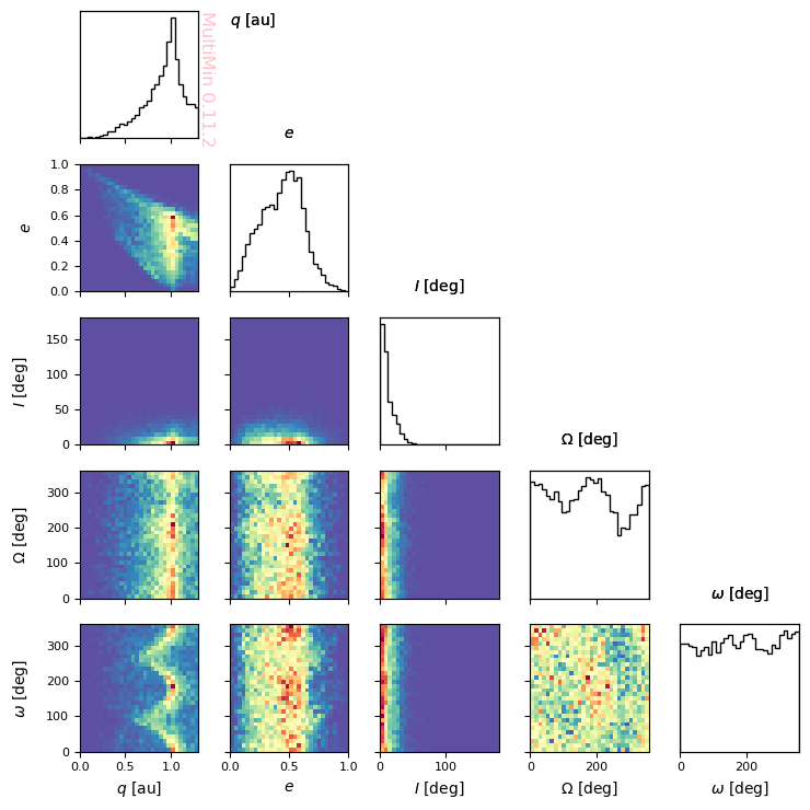
../_images/examples_multimin_density_plot_tutorial_18_0.png

[8]:

G=mn.MultiPlot(properties,figsize=1.5, marginals=True)

hargs=dict(bins=30,cmap='Spectral_r')
hist=G.sample_hist(data_neas,**hargs)

plt.savefig(f'gallery/{figprefix}_data_neas_hist.png')

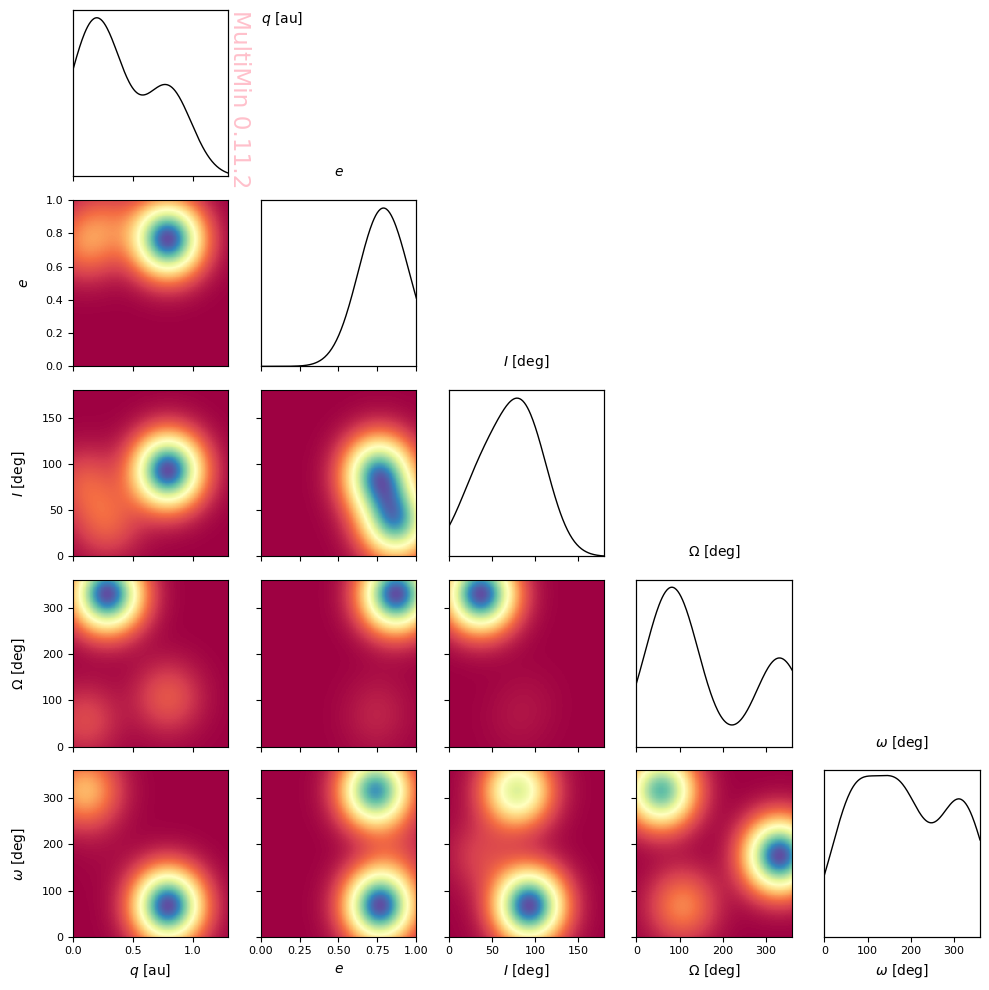
../_images/examples_multimin_density_plot_tutorial_19_0.png

You can also represent the pdf of some probability distribution. First, we generate a MoG:

[9]:

np.random.seed(5)
mus = np.array([[np.random.uniform(*properties[k]['range']) for k in properties] for _ in range(3)])
Sigmas = np.array([np.diag([(0.3 * np.mean(properties[k]['range']))**2 for k in properties]) for _ in range(3)])
mog = mn.MixtureOfGaussians(
    mus=mus,
    Sigmas=Sigmas,
    weights=[1]*3
)

Y ahora procedemos a graficarla:

[10]:

G=mn.MultiPlot(properties,figsize=2,marginals=True)

pargs = dict(cmap='Spectral')
G.mog_pdf(mog,**pargs)

plt.savefig(f'gallery/{figprefix}_sample_mog.png')

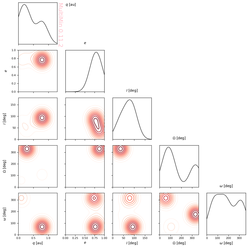
../_images/examples_multimin_density_plot_tutorial_23_0.png

You can also plot the contours:

[11]:

G=mn.MultiPlot(properties,figsize=2,marginals=True)

cargs = dict(levels=10)
G.mog_contour(mog,**cargs)

plt.savefig(f'gallery/{figprefix}_sample_mog_contours.png')

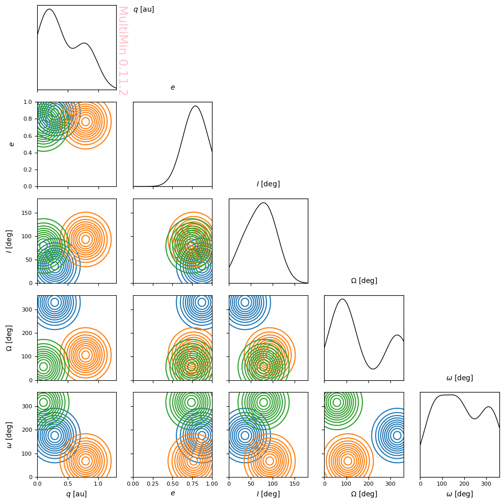
../_images/examples_multimin_density_plot_tutorial_25_0.png

Or isolate them:

[12]:

G=mn.MultiPlot(properties,figsize=2,marginals=True)

cargs = dict(levels=10, decomp=True, legend=False)
G.mog_contour(mog,**cargs)

plt.savefig(f'gallery/{figprefix}_sample_mog_contours_decomposed.png')

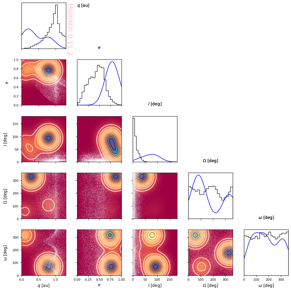
../_images/examples_multimin_density_plot_tutorial_27_0.png

Or put them together:

[13]:

G=mn.MultiPlot(properties,figsize=2,marginals=True)

sargs=dict(s=0.2,edgecolor='None',color='w')
scatter=G.sample_scatter(data_neas,**sargs)

pargs = dict(cmap='Spectral',margs=dict(color='b'))
G.mog_pdf(mog,**pargs)

cargs = dict(levels=10,margs=dict(color='b'))
G.mog_contour(mog,**cargs)

plt.savefig(f'gallery/{figprefix}_multiple_content.png')

../_images/examples_multimin_density_plot_tutorial_29_0.png

MultiMin - Multivariate Gaussian fitting