Mixture of Gaussians (MoG): A tutorial

This notebook gives a short introduction to MultiMin: fitting and visualizing Mixture of Gaussianss (MoG).

Installation and importing

If you’re running this in Google Colab or need to install the package, uncomment and run the following cell:

[1]:

try:
    from google.colab import drive
    %pip install -Uq multimin
except ImportError:
    print("Not running in Colab, skipping installation")
    %load_ext autoreload
    %autoreload 2
!mkdir -p gallery/

# Uncomment to install from GitHub (development version)
# !pip install git+https://github.com/seap-udea/MultiMin.git

Not running in Colab, skipping installation

[2]:

import multimin as mn
mn.show_watermark = True

import matplotlib.pyplot as plt
import plotly.graph_objects as go
from IPython.display import Markdown, display

import numpy as np
np.random.seed(1)
deg = np.pi/180

import warnings
warnings.filterwarnings("ignore")

figprefix = "mog"

Welcome to MultiMin v0.11.2. ¡Al infinito y más allá!

Theoretical background

The core of MultiMin is the Mixture of Gaussians (MoG) defined as:

\[\mathcal{C}_{M,k}(\tilde U; \{w_k\}_M, \{\mu_k\}_M, \{\Sigma_k\}_M) \equiv \sum_{i=1}^{M} w_i\mathcal{N}_k(\tilde U; \tilde \mu_i, \Sigma_i)\]

where \(\tilde U:(u_1,u_2,u_3,\ldots,u_N)\) are random variables and the multivariate normal distribution (MND) \(\mathcal{N}_k(\tilde U; \tilde \mu, \Sigma)\) with mean vector \(\tilde \mu\) and covariance matrix \(\Sigma\) is given by:

\[\mathcal{N}_k(\tilde U; \tilde \mu, \Sigma) = \frac{1}{\sqrt{(2\pi)^{k} \det \Sigma}} \exp\left[-\frac{1}{2}(\tilde U - \tilde \mu)^{\rm T} \Sigma^{-1} (\tilde U - \tilde \mu)\right]\]

The covariance matrix \(\Sigma_{k\times k}\) elements are defined as \(\Sigma_{ij} = \rho_{ij}\sigma_{i}\sigma_{j}\), where \(\sigma_i\) is the standard deviation of \(u_i\) and \(\rho_{ij}\) is the correlation coefficient between variable \(u_i\) and \(u_j\) (\(-1<\rho_{ij}<1\), \(\rho_{ii}=1\)).

The normalization condition implies that the set of weights \(\{w_k\}_M\) are also normalized, i.e., \(\sum_i w_i=1\).

Distribution basics

Below we define and visualize MoGs before using them for fitting.

Univariate normal distribution

The simplest case is a mixture of univariate normals. Here we create a MoG with two Gaussian components:

[3]:

MoG = mn.MixtureOfGaussians(
    mus=[0.0, 2.5],
    Sigmas=[1.0, 0.25],
    weights=[0.2, 0.8]
)

We can plot a sample from the distribution:

[4]:

G = MoG.plot_sample(
    properties=["x"],
    sargs=dict(s=0.5, alpha=0.5),
    figsize=3
)
plt.savefig(f'gallery/{figprefix}_univariate_sample_hist.png')

MixtureOfGaussians.rvs executed in 0.8513691425323486 seconds

../_images/examples_multimin_mog_tutorial_11_1.png

[5]:

MoG.update_params(
    weights=[0.5, 0.5],
)
G = MoG.plot_sample(
    properties=["x"],
    sargs=dict(s=0.5, alpha=0.5),
    figsize=3
)

MixtureOfGaussians.rvs executed in 0.7406923770904541 seconds

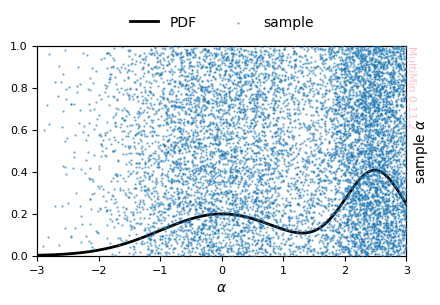
../_images/examples_multimin_mog_tutorial_12_1.png

Or you may specify in a more complex way the features of the properties:

[6]:

G = MoG.plot_sample(
    properties=dict(x=dict(label=r"$\alpha$", range=[-3,3])),
    sargs=dict(s=0.5, alpha=0.5),
    figsize=3
)
plt.savefig(f'gallery/{figprefix}_univariate_sample_hist.png')

MixtureOfGaussians.rvs executed in 0.8093640804290771 seconds

../_images/examples_multimin_mog_tutorial_14_1.png

Other methods available for this class:

[7]:

MoG.describe()


Available methods for this object/class
================================================
  copy()
    Return a copy of the object.

  drop()
    Drop one of the gaussians. Ex. mog.drop(0)

  get_function()
    Return the source code of ``mog(X)`` and an executable function (type='python'), or LaTeX code with parameters in \begin{array} (type='latex'). Ex. code, mog = MoG.get_function()

  pdf()
    Compute the PDF. Ex. mog.pdf([1.0, 0.5])

  plot_pdf()
    Plot only the PDF of the MoG.

  plot_sample()
    Plot a sample of the MoG. Ex. plot_sample(N=1000, sargs=dict(s=0.5))

  rvs()
    (sin descripción)

  sample_mog_likelihood()
    Compute the negative value of the logarithm of the likelihood of a sample. Ex. mog.sample_mog_likelihood(uparams, data=data, pmap=pmap)

  set_domain()
    Set the support domain for each variable (finite or infinite). Ex. set_domain([None, [0, 1], None])

  set_params()
    Set the properties of the MoG from flatten params. After setting it generate flattend stdcorr and normalize weights. Ex. set_params(params, nvars=2)

  set_sigmas()
    Set the value of list of covariance matrices. After setting Sigmas it update params and stdcorr. Ex. set_sigmas([[[1, 0.2], [0.2, 1]]])

  set_stdcorr()
    Set the properties of the MoG from flatten stdcorr. After setting it generate flattened params and normalize weights. Ex. set_stdcorr(stdcorr, nvars=2)

  tabulate()
    Build a table of MoG parameters: weights, means (mu_i), standard deviations (sigma_i), and correlations (rho_ij, i < j). Diagonal rho_ii are 1 by definition and omitted. Ex. df = MoG.tabulate(sort_by='weight')

  update_params()
    Update MoG parameters in-place using FitMoG-like syntax.

You can generate random samples with rvs:

[8]:

sample = MoG.rvs(5000)
sample[:10]

MixtureOfGaussians.rvs executed in 0.4020729064941406 seconds

[8]:

array([[-0.57475964],
       [ 0.51016492],
       [-0.96013615],
       [ 2.70690677],
       [-0.4472173 ],
       [-0.13701182],
       [-0.45402699],
       [ 2.86373214],
       [ 1.27706175],
       [ 0.37566416]])

You can evaluate the PDF at any point:

[9]:

MoG.pdf(1.3)

[9]:

0.10807882631874657

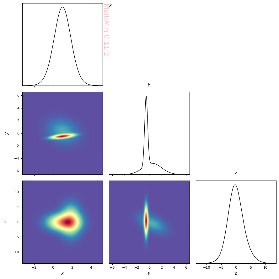
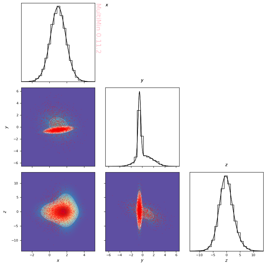
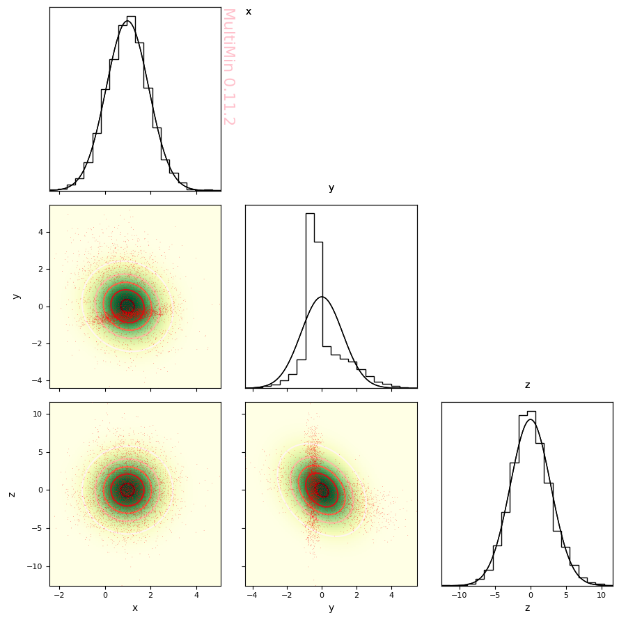
Multivariate distributions

The main strength of MultiMin is combining multivariate normal distributions. Below we define a MoG with two three-variate normals:

[10]:

weights = [0.5,0.5]
mus = [[1.0, 0.5, -0.5], [1.0, -0.5, +0.5],]
sigmas = [[1, 1.2, 2.3], [0.8, 0.2, 3.3]]
angles = [
    [10*deg, 30*deg, 20*deg],
    [-20*deg, 0*deg, 30*deg],
]
Sigmas = mn.Stats.calc_covariance_from_rotation(sigmas, angles)
MoG = mn.MixtureOfGaussians(mus=mus, weights=weights, Sigmas=Sigmas)

Preview the distribution with a 3D histogram:

[11]:

properties=dict(
    x=dict(label=r"$x$",range=None),
    y=dict(label=r"$y$",range=None),
    z=dict(label=r"$z$",range=None),
)

G = MoG.plot_pdf(
    properties=properties,
    figsize=3,
    grid_size=400,
    colorbar=False,
    cmap="Spectral_r",
    marginals=True,
)
plt.savefig(f'gallery/{figprefix}_3d_sample_density.png')

../_images/examples_multimin_mog_tutorial_25_0.png

Another way to visualize the distribution is with MultiPlot, which shows pairwise projections. We use a sample of the data:

[12]:

sample = MoG.rvs(5000)

MixtureOfGaussians.rvs executed in 0.6316561698913574 seconds

Plot the sample (2D histograms and scatter on the panels):

[13]:

G=mn.MultiPlot(properties,figsize=3, marginals=True)

G.mog_pdf(MoG)
G.mog_contour(MoG, levels=50, linewidth=0.1,alpha=0.3)

hargs=dict(bins=30,cmap='Spectral_r')
#hist=G.sample_hist(sample,**hargs)

sargs=dict(s=0.5,edgecolor='None',color='r')
hist=G.sample_scatter(sample,**sargs)

plt.savefig(f'gallery/{figprefix}_data_density_scatter.png')

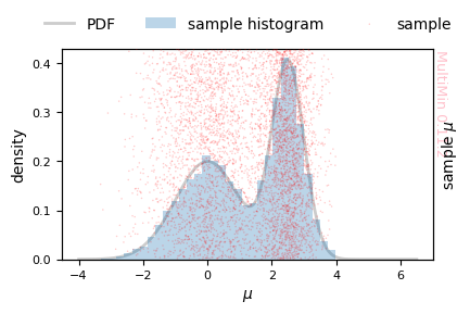
../_images/examples_multimin_mog_tutorial_29_0.png

MultiPlot can also be used for univariate distributions (single-panel histogram and scatter):

[14]:

MoG = mn.MixtureOfGaussians(
    mus=[0.0, 2.5],
    Sigmas=[1.0, 0.25],
    weights=[0.5, 0.5]
)

sample = MoG.rvs(5000)

properties=dict(
    x=dict(label=r"$\mu$",range=None),
)

G=mn.MultiPlot(properties,figsize=3)

G.mog_pdf(MoG, alpha=0.2)

G.sample_hist(
    sample,
    **dict(bins=30,cmap='Spectral_r', alpha=0.3),
)

sargs=dict(s=1.2,edgecolor='None',color='r')
G.sample_scatter(
    sample,
    **dict(s=1.2,edgecolor='None',color='r',alpha=0.2),
)
plt.savefig(f'gallery/{figprefix}_univariate_density_2gauss.png')

MixtureOfGaussians.rvs executed in 0.31572604179382324 seconds

../_images/examples_multimin_mog_tutorial_31_1.png

Fitting data with MoG

We fit by minimizing the negative normalized log-likelihood

\[-\frac{\log \mathcal{L}}{S} = -\frac{1}{S} \sum_{i=1}^{S} \log \mathcal{C}_M(\tilde{U}_i)\]

over the MoG parameters. Lower values indicate a better fit.

This notebook demonstrates how to use the multimin.multimin module for handling multidimensional distributions, specifically designed for asteroid population analysis.

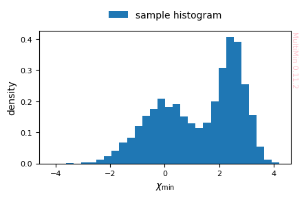
Univariate normals

The goal of MultiMin is to fit a MoG to a given dataset. We start with a univariate example by generating data from a MoG and then fitting it:

[15]:

# Create the distribution
MoG = mn.MixtureOfGaussians(
    mus=[0.0, 2.5],
    Sigmas=[1.0, 0.25],
    weights=[0.5, 0.5]
)

# Generate data
sample = MoG.rvs(10000)

# Plot the data
G = mn.MultiPlot(dict(x=dict(label=r"$\chi_\mathrm{min}$",range=None)),figsize=3)
G.sample_hist(sample,**dict(bins=30))
plt.savefig(f'gallery/{figprefix}_univariate_histogram.png')

MixtureOfGaussians.rvs executed in 0.6484818458557129 seconds

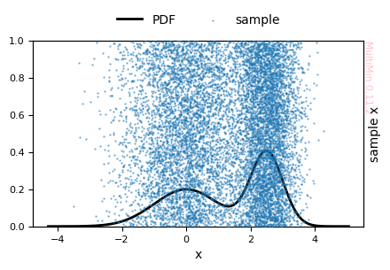
../_images/examples_multimin_mog_tutorial_35_1.png

Fit with a single Gaussian component:

[16]:

F = mn.FitMoG(data=sample, ngauss=1)

Loading a FitMoG object.
Number of gaussians: 1
Number of variables: 1
Number of dimensions: 1
Number of samples: 10000
Log-likelihood per point (-log L/N): 2.2970198330802165

Run the fitting procedure (use progress="tqdm" for better convergence):

[17]:

F.fit_data(progress="tqdm")

FitMoG.fit_data executed in 0.13362908363342285 seconds

Plot the fit result (histogram of data and fitted PDF):

[18]:

# Univariate: hargs → histogram of sample; fit shown as PDF
F.plot_fit(
    properties=["u"],
    hargs=dict(bins=30),
    sargs=dict(s=0.5,edgecolor='None',color='r'),
    pargs=dict(color='b'),
    figsize=3
)
plt.savefig(f'gallery/{figprefix}_univariate_fit_1gauss.png')

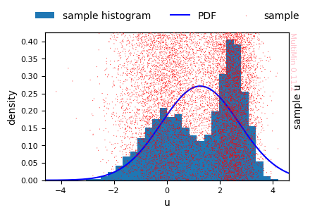
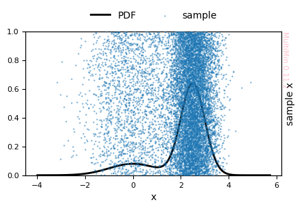
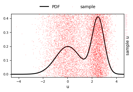
../_images/examples_multimin_mog_tutorial_41_0.png

A single Gaussian cannot capture the bimodal shape.

Fitting with two Gaussians:

[19]:

F = mn.FitMoG(data=sample, ngauss=2)
F.fit_data()
print(f"Log-likelihood per point (-log L/N) after fit: ",F.norm_log_l())
# Univariate: no hargs → scatter of sample; fit shown as PDF
F.plot_fit(
    properties=["u"],
    sargs=dict(s=0.5, edgecolor='None', color='r'),
    figsize=3
)
plt.savefig(f'gallery/{figprefix}_univariate_fit_2gauss.png')

Loading a FitMoG object.
Number of gaussians: 2
Number of variables: 1
Number of dimensions: 2
Number of samples: 10000
Log-likelihood per point (-log L/N): 2.2970198330802165
FitMoG.fit_data executed in 0.09199881553649902 seconds
Log-likelihood per point (-log L/N) after fit:  1.635612507663419

../_images/examples_multimin_mog_tutorial_44_1.png

Visual inspection shows that the fitted distribution matches the sample well. For a quantitative check we can compare the true and fitted parameters:

[20]:

MoG.tabulate('distance')

[20]:

	w	mu_1	sigma_1
component
1	0.5	0.0	1.00
2	0.5	2.5	0.25

[21]:

F.mog.tabulate('distance')

[21]:

	w	mu_1	sigma_1
component
2	0.500526	0.025683	1.004006
1	0.499474	2.508023	0.244823

The tables confirm that the fitted parameters are close to the true ones.

You can export the fitted MoG as a callable function for use in other code:

[22]:

code, mog = F.mog.get_function()

from multimin import Util

def mog(X):

    mu1_1 = 2.508023
    sigma1_1 = 0.494796
    n1 = Util.nmd(X, mu1_1, sigma1_1)

    mu2_1 = 0.025683
    sigma2_1 = 1.002001
    n2 = Util.nmd(X, mu2_1, sigma2_1)

    w1 = 0.499474
    w2 = 0.500526

    return (
        w1*n1
        + w2*n2
    )

Evaluate the fitted PDF at a point:

[23]:

mog(0.2)

[23]:

np.float64(0.1962968566936807)

Multivariate data

We can run a similar workflow for multivariate data:

[24]:

weights = [0.5,0.5]
mus = [[1.0, 0.5, -0.5], [1.0, -0.5, +0.5],]
sigmas = [[1, 1.2, 2.3], [0.8, 0.2, 3.3]]
angles = [
    [10*deg, 30*deg, 20*deg],
    [-20*deg, 0*deg, 30*deg],
]
Sigmas = mn.Stats.calc_covariance_from_rotation(sigmas, angles)

MoG = mn.MixtureOfGaussians(mus=mus, weights=weights, Sigmas=Sigmas)

sample = MoG.rvs(5000)

MixtureOfGaussians.rvs executed in 0.43866991996765137 seconds

First, fit with a single multivariate normal:

[25]:

F = mn.FitMoG(data=sample, ngauss=1)
F.fit_data(progress="tqdm")

Loading a FitMoG object.
Number of gaussians: 1
Number of variables: 3
Number of dimensions: 3
Number of samples: 5000
Log-likelihood per point (-log L/N): 11.414133112430706

FitMoG.fit_data executed in 0.1270902156829834 seconds

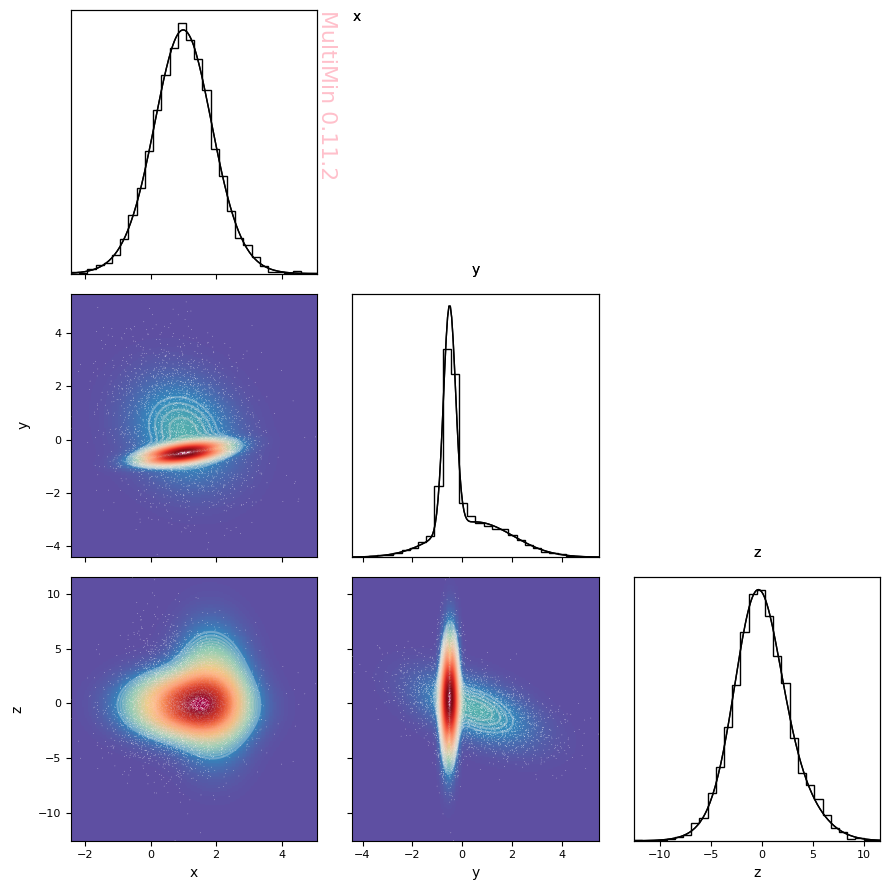
Check the fit (one Gaussian cannot capture two modes):

[26]:

G=F.plot_fit(
    properties=["x","y","z"],
    sargs=dict(s=0.2,edgecolor='None',color='r'),
    pargs=dict(cmap='YlGn'),
    cargs=dict(),
    figsize=3,
    marginals=True,
)

plt.savefig(f'gallery/{figprefix}_fit_2gauss_3d.png')

../_images/examples_multimin_mog_tutorial_59_0.png

Although we can evaluate visually that the fit is not good, we can better check the goodness of fit using a Kolmogorov-Smirnov test.

[27]:

ks, R2 = F.quality_of_fit(plot_qq=True)
plt.savefig(f"gallery/{figprefix}_plot_qq_mog.png")

MixtureOfGaussians.rvs executed in 2.660444974899292 seconds

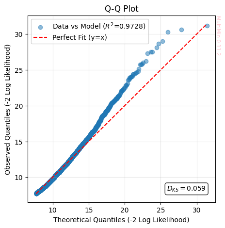
../_images/examples_multimin_mog_tutorial_61_1.png

the Kolmogorov-Smirnov Statistic (:math:`D_{KS}`) Measures the maximum absolute distance between the Cumulative Distribution Function (CDF) of the data and that of the model. It represents the “worst point” of local deviation.

\[D_{KS} = \sup_{x} | F_{obs}(x) - F_{model}(x) |\]

The range of the statistics is \(D_{KS}\in[0, 1]\), where an acceptable value is \(D_{KS}\approx 0\) (Ideally \(< 0.05\)).

The Q-Q plot is a non-parametric visual diagnostic tool used to assess whether a set of observed data follows a specific theoretical distribution (or a model simulation). For making it we compare the distribution of the Negative Log-Likelihood (\(-\ln \mathcal{L}\)) of the real data against the model’s prediction. The plot confronts the quantiles of the empirical distribution (data) against the quantiles of the reference distribution (model).

If two distributions \(F_{obs}\) and \(F_{model}\) are identical, then for any probability \(p\), their inverses (the quantiles) must match. Therefore, the points \((x, y) = (Q_{model}, Q_{obs})\) should align on the identity line \(y = x\). Since visualizing an \(N\)-dimensional space is impossible for humans, we use the Log-Likelihood as a dimensionality reduction technique. We collapse the vector \(\vec{x}\) into a scalar \(S = -2 \ln \mathcal{L}(\vec{x})\). If the Q-Q plot of \(S\) is correct, we have strong assurance that the model correctly captures the internal correlations and structure of the n-tuples.

Ideal Fit (On the :math:`y=x` line): The distribution of “rarity” in the observed events perfectly matches the model’s prediction. The fit is statistically valid.
Tail Deviation (Curved ends): Points diverging at the extremes (top right or bottom left) indicate “Heavy Tails” (more outliers than predicted) or “Light Tails” (fewer outliers than predicted).
Shift or Wrong Slope: Indicates systematic errors in the mean (displacement) or variance (scale) of the model.

The Coefficient of Determination on Identity (:math:`R^2`) measures the variance explained by the model with respect to the ideal line \(y=x\). It penalizes both dispersion and bias (displacement) of the prediction.

\[R^2 = 1 - \frac{\sum (y_{obs} - x_{model})^2}{\sum (y_{obs} - \bar{y}_{obs})^2}\]

The range of the statistics is \(R^2\in(-\infty, 1]\), where an acceptable value is \(R^2\approx 1\) (Ideally \(> 0.9\)).

In all the metrics, the fit to a single gaussian is poor for the considered data.

Fitting with two Gaussians gives a much better result:

[28]:

F = mn.FitMoG(data=sample, ngauss=2)
F.fit_data(progress="tqdm")
G=F.plot_fit(
    properties=["x","y","z"],
    pargs=dict(cmap='Spectral_r'),
    sargs=dict(s=0.2,edgecolor='None',color='w',nbins=30),
    cargs=dict(levels=50,zorder=+300,alpha=0.3),
    figsize=3,
    marginals=True
)

plt.savefig(f'gallery/{figprefix}_fit_result_3d.png')

Loading a FitMoG object.
Number of gaussians: 2
Number of variables: 3
Number of dimensions: 6
Number of samples: 5000
Log-likelihood per point (-log L/N): 11.414133112430706

FitMoG.fit_data executed in 0.5385608673095703 seconds

../_images/examples_multimin_mog_tutorial_65_3.png

Much better! At least visually. Let’s evaluate the quality of fit quantitatively.

[29]:

ks, R2 = F.quality_of_fit(plot_qq=True)
plt.savefig(f"gallery/{figprefix}_plot_qq_mog_full.png")

MixtureOfGaussians.rvs executed in 3.3428080081939697 seconds

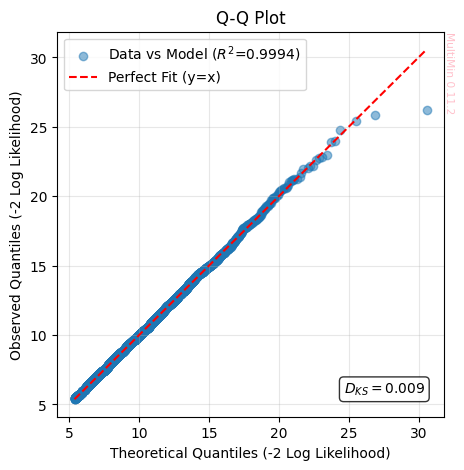
../_images/examples_multimin_mog_tutorial_67_1.png

Wonderful!

Check the initial and final distributions:

Compare the true and fitted MoG parameters (e.g. means and weights):

[30]:

MoG.tabulate('distance')

[30]:

	w	mu_1	mu_2	mu_3	sigma_1	sigma_2	sigma_3	rho_12	rho_13	rho_23
component
1	0.5	1.0	0.5	-0.5	1.064392	1.510773	2.077169	-0.211137	0.101191	-0.534075
2	0.5	1.0	-0.5	0.5	0.788611	0.241023	3.300000	0.539822	0.000000	0.000000

[31]:

F.mog.tabulate('distance')

[31]:

	w	mu_1	mu_2	mu_3	sigma_1	sigma_2	sigma_3	rho_12	rho_13	rho_23
component
2	0.503237	1.001685	-0.504055	0.534949	0.788532	0.241555	3.349363	0.529687	-0.008064	0.046706
1	0.496763	0.977029	0.528189	-0.558262	1.059248	1.517444	2.067635	-0.205607	0.090194	-0.530379

The agreement is as expected for a good fit.

You can obtain the fitted PDF as explicit code or a callable:

[32]:

code, pymog = F.mog.get_function(cmog=False)

from multimin import Util

def mog(X):

    mu1_1 = 0.977029
    mu1_2 = 0.528189
    mu1_3 = -0.558262
    mu1 = [mu1_1, mu1_2, mu1_3]
    Sigma1 = [[1.122005, -0.330481, 0.197538], [-0.330481, 2.302636, -1.664074], [0.197538, -1.664074, 4.275116]]
    n1 = Util.nmd(X, mu1, Sigma1)

    mu2_1 = 1.001685
    mu2_2 = -0.504055
    mu2_3 = 0.534949
    mu2 = [mu2_1, mu2_2, mu2_3]
    Sigma2 = [[0.621782, 0.100891, -0.021299], [0.100891, 0.058349, 0.037788], [-0.021299, 0.037788, 11.218229]]
    n2 = Util.nmd(X, mu2, Sigma2)

    w1 = 0.496763
    w2 = 0.503237

    return (
        w1*n1
        + w2*n2
    )

LaTeX outputs

For papers or reports you can export the fitted function in LaTeX:

[33]:

function, _ = F.mog.get_function(type='latex')
display(Markdown(function))

$$f(\mathbf{x}) = w_1 \, \mathcal{N}(\mathbf{x}; \boldsymbol{\mu}_1, \mathbf{\Sigma}_1) + w_2 \, \mathcal{N}(\mathbf{x}; \boldsymbol{\mu}_2, \mathbf{\Sigma}_2)$$

where

$$w_1 = 0.496763$$
$$\boldsymbol{\mu}_1 = \left( \begin{array}{c} 0.977029 \\ 0.528189 \\ -0.558262 \end{array}\right)$$
$$\mathbf{\Sigma}_1 = \left( \begin{array}{ccc} 1.122005 & -0.330481 & 0.197538 \\ -0.330481 & 2.302636 & -1.664074 \\ 0.197538 & -1.664074 & 4.275116 \end{array}\right)$$

$$w_2 = 0.503237$$
$$\boldsymbol{\mu}_2 = \left( \begin{array}{c} 1.001685 \\ -0.504055 \\ 0.534949 \end{array}\right)$$
$$\mathbf{\Sigma}_2 = \left( \begin{array}{ccc} 0.621782 & 0.100891 & -0.021299 \\ 0.100891 & 0.058349 & 0.037788 \\ -0.021299 & 0.037788 & 11.218229 \end{array}\right)$$

Here the normal distribution is defined as:

$$\mathcal{N}(\mathbf{x}; \boldsymbol{\mu}, \mathbf{\Sigma}) = \frac{1}{\sqrt{(2\pi)^{{k}} \det \mathbf{\Sigma}}} \exp\left[-\frac{1}{2}(\mathbf{x}-\boldsymbol{\mu})^{\top} \mathbf{\Sigma}^{{-1}} (\mathbf{x}-\boldsymbol{\mu})\right]$$

\[f(\mathbf{x}) = w_1 \, \mathcal{N}(\mathbf{x}; \boldsymbol{\mu}_1, \mathbf{\Sigma}_1) + w_2 \, \mathcal{N}(\mathbf{x}; \boldsymbol{\mu}_2, \mathbf{\Sigma}_2)\]

where

\[w_1 = 0.496763\]

\[\begin{split}\boldsymbol{\mu}_1 = \left( \begin{array}{c} 0.977029 \\ 0.528189 \\ -0.558262 \end{array}\right)\end{split}\]

\[\begin{split}\mathbf{\Sigma}_1 = \left( \begin{array}{ccc} 1.122005 & -0.330481 & 0.197538 \\ -0.330481 & 2.302636 & -1.664074 \\ 0.197538 & -1.664074 & 4.275116 \end{array}\right)\end{split}\]

\[w_2 = 0.503237\]

\[\begin{split}\boldsymbol{\mu}_2 = \left( \begin{array}{c} 1.001685 \\ -0.504055 \\ 0.534949 \end{array}\right)\end{split}\]

\[\begin{split}\mathbf{\Sigma}_2 = \left( \begin{array}{ccc} 0.621782 & 0.100891 & -0.021299 \\ 0.100891 & 0.058349 & 0.037788 \\ -0.021299 & 0.037788 & 11.218229 \end{array}\right)\end{split}\]

Here the normal distribution is defined as:

\[\mathcal{N}(\mathbf{x}; \boldsymbol{\mu}, \mathbf{\Sigma}) = \frac{1}{\sqrt{(2\pi)^{{k}} \det \mathbf{\Sigma}}} \exp\left[-\frac{1}{2}(\mathbf{x}-\boldsymbol{\mu})^{\top} \mathbf{\Sigma}^{{-1}} (\mathbf{x}-\boldsymbol{\mu})\right]\]

You can also output the parameter table in LaTeX:

[34]:

latex_table = F.mog.tabulate(type='latex')

\begin{table*}
\begin{tabular}{lrrrrrrrrrr}
\hline
$k$ & $w$ & $\mu_{1}$ & $\mu_{2}$ & $\mu_{3}$ & $\sigma_{1}$ & $\sigma_{2}$ & $\sigma_{3}$ & $\rho_{12}$ & $\rho_{13}$ & $\rho_{23}$ \\
\hline
2 & 0.5032 & 1.002 & -0.5041 & 0.5349 & 0.7885 & 0.2416 & 3.349 & 0.5297 & -0.008064 & 0.04671 \\
1 & 0.4968 & 0.977 & 0.5282 & -0.5583 & 1.059 & 1.517 & 2.068 & -0.2056 & 0.09019 & -0.5304 \\
\hline
\end{tabular}
\end{table*}

MultiMin - Multivariate Gaussian fitting